Octave Convolution: Taking a step back and at looking inputs ?

Convolutional neural networks (CNNs) have dominated the field of computer vision. In this post, we shall look at the recently proposed Octave convolution from this paper: Drop an Octave: Reducing Spatial Redundancy in Convolutional Neural Networks with Octave Convolution.
Octave convolution can be used as a replacement for vanilla convolution. It has been demonstrated by the authors that similar (sometimes better) accuracy can be achieved using octave convolution while saving a huge number of flops required. Model size in case of octave and vanilla convolutions is same.
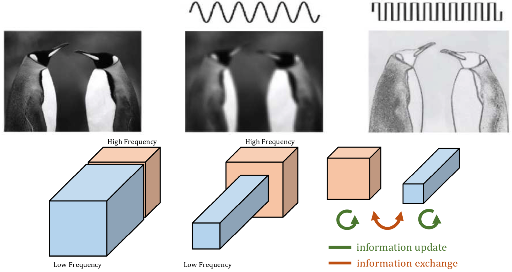
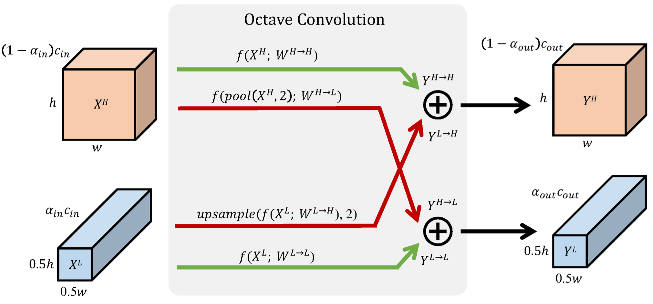
Vanilla convolution carries out high frequency convolution throughout all the inputs channels. Octave convolution on the other hand, partitions all channels into two parts: high frequency and low frequency. Low frequency channels are one octave smaller (height and width) compared to high frequency convolutions. Moreover, high and low frequency channels are combined with each other before sending out the outputs.
As can be seen in the figure, each octave convolution module can have upto 4 branches inside it each doing vanilla convolution. The paths with green color, donot change the spatial dimensions going from input to output. However, the paths with red color either increase (Low-to-high) or decrease (High-to-low) the spatial dimensions going from input to output.
When going from high frequency input to low frequency output (HtoL path), a 2x2 pooling operation is done to get the downscaled input for convolution. So, the HtoL path is conv_vanilla(pool(in_high))
Similarly when going from Low Frequency input to high frequency output (LtoH path), a vanilla convolution is topped with a bilinear interpolation to upsample the low resolution conv output. So, the LtoH path is bilenear_interpolation(vanilla_convolution(in_low)).

At the heart of Octave convolution lies the concept of $\alpha$ (ratio of the total channels which are used by low frequency convolutions). For the first convolution layer, there is no low frequency input channel, so $\alpha_{in} = 0$. Similarly for the last convolution layer, there is no low frequency output channel, $\alpha_{out} = 0$. For all the other layers, the authors assumed $\alpha_{in} = \alpha_{out} = 0.5$.
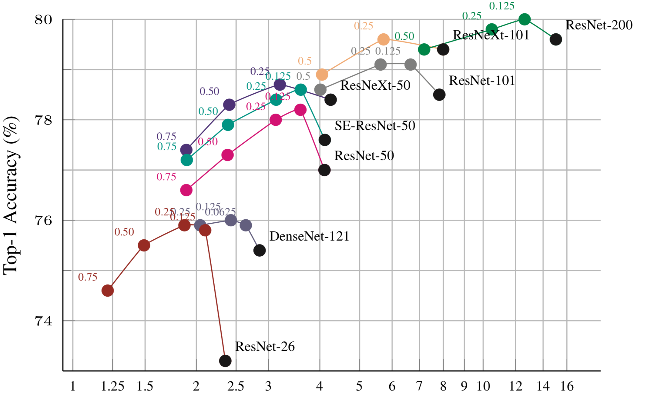
The authors showed a lot of results in the paper. The one I find most interesting is shown below. As you can see, with a small portion of low frequency component (0.125 or 0.25), the networks perform better than the baseline models with all high-frequency channels.

Following is a Pytorch implementation.
class OctConv(nn.Module):
    def __init__(self, ch_in, ch_out, kernel_size, stride=1, alphas=[0.5,0.5]):
        super(OctConv, self).__init__()

        # Get layer parameters
        self.alpha_in, self.alpha_out = alphas
        assert 0 <= self.alpha_in <= 1 and 0 <= self.alpha_in <= 1, \
        			"Alphas must be in interval [0, 1]"
        self.kernel_size = kernel_size
        self.stride = stride
        self.padding = (kernel_size - stride ) // 2

        # Calculate the exact number of high/low frequency channels
        self.ch_in_lf = int(self.alpha_in*ch_in)
        self.ch_in_hf = ch_in - self.ch_in_lf
        self.ch_out_lf = int(self.alpha_out*ch_out)
        self.ch_out_hf = ch_out - self.ch_out_lf

        # Create convolutional and other modules necessary. Not all paths
        # will be created in call cases. So we check number of high/low freq
        # channels in input/output to determine which paths are present.
        # Example: First layer has alpha_in = 0, so hasLtoL and hasLtoH (bottom
        # two paths) will be false in this case.
        self.hasLtoL = self.hasLtoH = self.hasHtoL = self.hasHtoH = False
        if (self.ch_in_lf and self.ch_out_lf):
          	# Green path at bottom.
            self.hasLtoL = True
            self.conv_LtoL = nn.Conv2d(self.ch_in_lf, self.ch_out_lf, \
                                       self.kernel_size, padding=self.padding)
        if (self.ch_in_lf and self.ch_out_hf):
          	# Red path at bottom.
            self.hasLtoH = True
            self.conv_LtoH = nn.Conv2d(self.ch_in_lf, self.ch_out_hf, \
                                       self.kernel_size, padding=self.padding)
        if (self.ch_in_hf and self.ch_out_lf):
          	# Red path at top
            self.hasHtoL = True
            self.conv_HtoL = nn.Conv2d(self.ch_in_hf, self.ch_out_lf, \
                                       self.kernel_size, padding=self.padding)
        if (self.ch_in_hf and self.ch_out_hf):
          	# Green path at top
            self.hasHtoH = True
            self.conv_HtoH = nn.Conv2d(self.ch_in_hf, self.ch_out_hf, \
                                       self.kernel_size, padding=self.padding)
        self.avg_pool  = nn.AvgPool2d(2,2)

    def forward(self, input):
        # Split input into high frequency and low frequency components
        fmap_w = input.shape[-1]
        fmap_h = input.shape[-2]
        # We resize the high freqency components to the same size as the low
        # frequency component when sending out as output. So when bringing in as
        # input, we want to reshape it to have the original size as the intended
        # high frequnecy channel (if any high frequency component is available).
        input_hf = input
        if (self.ch_in_lf):
            input_hf = input[:,:self.ch_in_hf*4,:,:].reshape(-1, \
                                       self.ch_in_hf,fmap_h*2,fmap_w*2)
            input_lf = input[:,self.ch_in_hf*4:,:,:]

        # Create all conditional branches
        LtoH = HtoH = LtoL = HtoL = 0.
        if (self.hasLtoL):
          	# Since, there is no change in spatial dimensions between input and
            # output, we use vanilla convolution
            LtoL = self.conv_LtoL(input_lf)
        if (self.hasHtoH):
          	# Since, there is no change in spatial dimensions between input and
            # output, we use vanilla convolution
            HtoH = self.conv_HtoH(input_hf)
            # We want the high freq channels and low freq channels to be
            # packed together such that the output has one dimension. This
            # enables octave convolution to be used as is with other layers
            # like Relu, elementwise etc. So, we fold the high-freq channels
            # to make its height and width same as the low-freq channels. So,
            # h = h/2 and w = w/2 since we are making h and w smaller by a
            # factor of 2, the number of channels increases by 4.
            op_h, op_w = HtoH.shape[-2]//2, HtoH.shape[-1]//2
            HtoH = HtoH.reshape(-1, self.ch_out_hf*4, op_h, op_w)
        if (self.hasLtoH):
          	# Since, the spatial dimension has to go up, we do
            # bilinear interpolation to increase the size of output
            # feature maps
            LtoH = F.interpolate(self.conv_LtoH(input_lf), \
                                 scale_factor=2, mode='bilinear')
            # We want the high freq channels and low freq channels to be
            # packed together such that the output has one dimension. This
            # enables octave convolution to be used as is with other layers
            # like Relu, elementwise etc. So, we fold the high-freq channels
            # to make its height and width same as the low-freq channels. So,
            # h = h/2 and w = w/2 since we are making h and w smaller by a
            # factor of 2, the number of channels increases by 4.
            op_h, op_w = LtoH.shape[-2]//2, LtoH.shape[-1]//2
            LtoH = LtoH.reshape(-1, self.ch_out_hf*4, op_h, op_w)
        if (self.hasHtoL):
          	# Since, the spatial dimension has to go down here, we do
            # average pooling to reduce the height and width of output
            # feature maps by a factor of 2
            HtoL = self.avg_pool(self.conv_HtoL(input_hf))

        # Elementwise addition of high and low freq branches to get the output
        out_hf = LtoH + HtoH
        out_lf = LtoL + HtoL

        # Since, not all paths are always present, we need to put a check
        # on how the output is generated. Example: the final convolution layer
        # will have alpha_out == 0, so no low freq. output channels,
        # so the layers returns just the high freq. components. If there are no
        # high freq component then we send out the low freq channels (we have it
        # just to have a general module even though this scenerio has not been
        # used by the authors). If both low and high freq components are present,
        # we concat them (we have already resized them to be of the same dimension)
        # and send them out.
        if (self.ch_out_lf == 0):
            return out_hf
        if (self.ch_out_hf == 0):
            return out_lf
        op = torch.cat([out_hf,out_lf],dim=1)
        return op
Complete implementation can be found at my git repo. For testing this implementation, I trained a 2 layer vanilla CNN on CIFAR10 for some 20 epochs. Then I replaced all convolutions with Octave convolution. the network performed slightly better (2-3%). I feel, for bigger networks the difference might be even better.