The Subtle Art of Fixing and Modifying Learning Rate
Learning rate is one of the most critical hyper-parameters and has the potential to decide the fate of your deep learning algorithm. If you mess it up, then the optimizer might not be able to converge at all! It acts as a gate which controls how much the optimizer is updating the parameters wrt gradient of loss. Speaking in terms of equations, gradient is given by:
Using this gradient from the minibatch, stochastic gradient descent follows the estimated downhill:
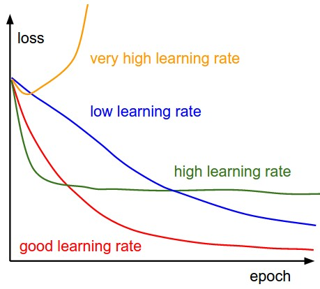
where is the learning rate. The following figure explains the effects of learning rate on gradient descent. A very small learning rate will make gradient descent take small steps even if the gradient is big, thus slowing the process of learning. If the learning rate is high, then if becomes impossible to learn very small changes in the parameters needed to fine tune the model towards the end of the training process, so the error flattens out very early. If the learning rate is very high, then gradient descent takes big steps and jumps around. This can lead to divergence and thus increase the error.
Selecting a good starting value for learning rate
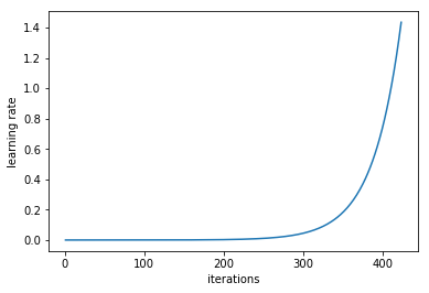
Now the question aries, what is the best value of the learning rate and how to decide it ? A systematic way to estimate a good learning rate is by training the model initially with a very low learning rate and increasing it (either linearly or exponentially) at each iteration (illustrated below). We keep doing it to the point where the loss stops decreasing and starts to increase. That means that the learning rate is too high for the application and so gradient descent is diverging. For practical applications our learning rate should ideally be 1 or 2 step smaller than this value.
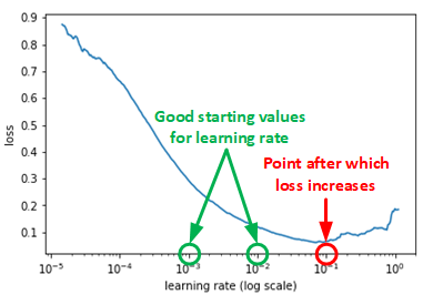
If we keep track of the learning rate and plot log of the learning rate and the error we will see a plot as shown below. A good learning rate somewhere to the left to the lowest point of the graph (as demonstrated in below graph). In this case, its 0.001 to 0.01.
In general no fixed learning rate works best for the entire training process. Typically we start with a learning rate found using the method described above. During the training process we change learning rate to best facilitate learning. There are many different ways to accomplish this. In this blog, we will go through a few popular learning rate scheduler.
Step Decay
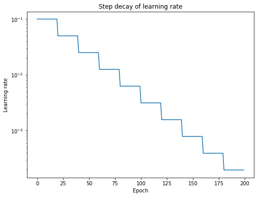
Step decay schedule drops the learning rate by a factor every few epochs. Mathematical form of step decay is:
where, is the learning rate for epoch, is the initial learning rate, is the fraction by which learning rate is reduced, is floor operation and N is the number of epochs after which learning rate is dropped.
In tensorflow this can be done easily. To modify the learning rate we need a variable to store the learning rate and a variable to store the number of iterations.
...
global_step = tf.Variable(0, trainable=False)       # Variable to store number of iterations
starter_learning_rate = 0.1                         # Initial Learning rate
learning_rate = tf.train.exponential_decay(
                starter_learning_rate, global_step,  # Function applied by TF on the varible (same formula as shown above)
                100000, 0.96, staircase=True)        # make staircase=True to force an integer division and thus create a step decay
# Passing global_step to minimize() will increment it at each step.
learning_step = (
    tf.train.GradientDescentOptimizer(learning_rate)        # We create an instance of the optimizer with updated learning rate each time
    .minimize(...my loss..., global_step=global_step)       # global step (# iterations) is updated by the minimize function
)
Linear or Exponential Time-Based Decay
This technique is also known as learning rate annealing. We start with a relatively high learning rate and then gradually lower it during training. The intuition behind this approach is that we’d like to traverse quickly from the initial parameters to a range of “good” parameter values but then we’d like a learning rate small enough that we can explore the “deeper, but narrower parts of the loss function” (fine tuning the parameters to get best results).
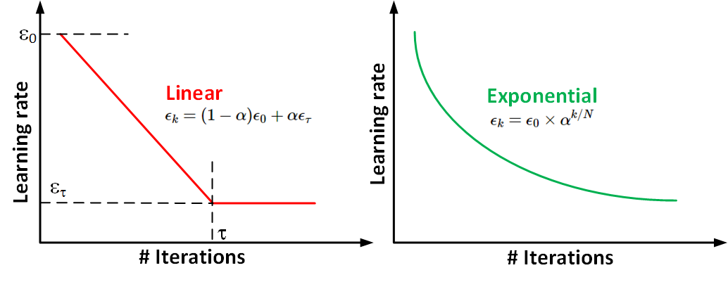
In practice, it is common to decay the learning rate until iteration . In case of linear decay, the learning rate is modified in the following manner:
with . After iteration , it is common to leave constant.
In case of exponential decay:
In tensorflow this can be implemented like we implemented step decay. In this case, we make staircase=False, this uses a floating division and thus leads to gradual decrease in learning rate.
...
global_step = tf.Variable(0, trainable=False)
starter_learning_rate = 0.1
learning_rate = tf.train.exponential_decay(
                    starter_learning_rate, global_step,
                    100000, 0.96, staircase=False)   # make staircase=False to force an float division and thus create a gradual decay
# Passing global_step to minimize() will increment it at each step.
learning_step = (
    tf.train.GradientDescentOptimizer(learning_rate)
    .minimize(...my loss..., global_step=global_step)
)
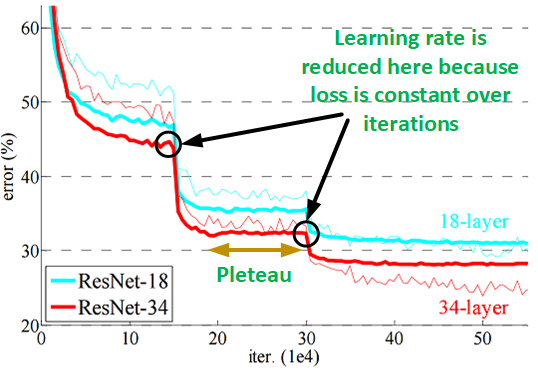
Decrease learning rate when you hit a pleteau
This technique is also very popular and its intuitive also. Keep using a big learning rate to quickly appraoch a local minima and reduce it once we hit a plateau (i.e. this learning rate is too big for now, we need smaller value to be able to fine tune the parameters more). The term plateau referes to the point when the change in loss wrt training iterations is less then a threshold . What it essentially means is the loss vs iterations curve becomes flat. This is illustrated in the figure below.
These sort of custom learning rate decay scheduler can be easily impelemented by making the learning rate a placeholder. We then calculate the learning rate based on some set of rules and pass it to tensorflow in the feed_dict along with other data (input, output, dropout ratio, etc).
loss_over_last_N_iters = [] # Keep track of loss in last N iterations
lr = 0.01 # can be anything
for global_step in range(0,total_steps):
    learning_rate = tf.placeholder(tf.float32, shape=[])
    change_in_loss = get_loss_change(loss_over_last_N_iters) # determine if the loss is changing or has hit a plateau.
    if change_in_loss > theta:
        lr = lr*alpha   # Change the learning rate (eg. make it lr/10)
    # ...
    loss = ...
    train_step = tf.train.GradientDescentOptimizer(
        learning_rate=learning_rate).minimize(mse)  # create an optimizer with the placeholder input as learning rate
    sess = tf.Session()

    # Feed different values for learning rate to each training step.
    error, _ = sess.run([loss, train_step], feed_dict={learning_rate: lr, data: ...})  # pass the rule based lr in feed dict

    loss_over_last_N_iters.append(0,error)      # Get the new loss and update the list tracking loss
    loss_over_last_N_iters.pop()
Cyclic learning rates
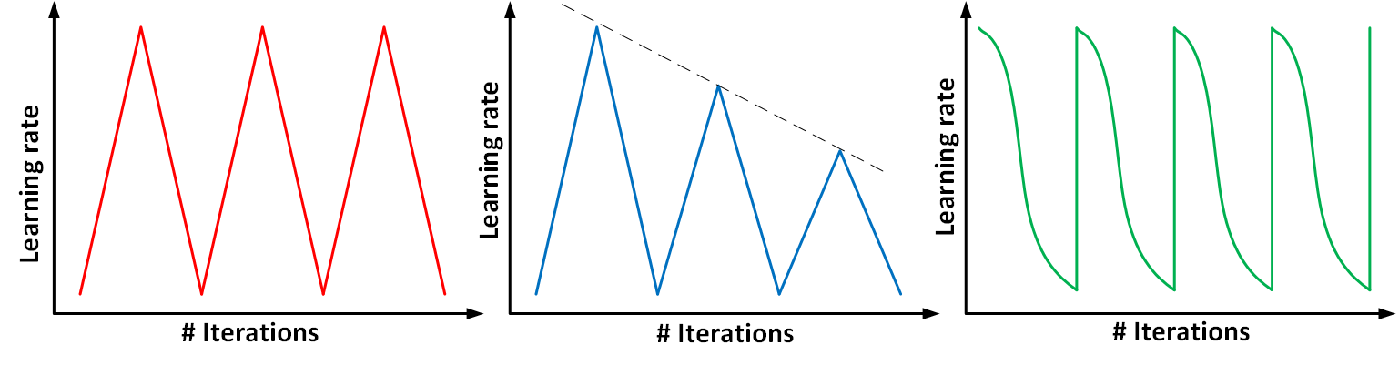
All the schemes we discussed so far were targeted at starting with a large learning rate and making it smaller as training progressed. some works like Cyclical Learning Rates for Training Neural Networks and Stochastic Gradient Descent with Warm Restarts suggest otherwise. The underlying assumption behind cyclic learning rate is “ increasing the learning rate might have a short term negative effect and yet achieve a longer term beneficial effect”. The authors of these works have demonstrated that a cyclical learning rate schedule which varies between two bound values can deliver results better than the traditional learning rate schedules. The intuition behind why cyclic learning rates work are:
- A minima that generalizes data well should not be a sharp minima, i.e. slight change in the parameters should not degrade the performance. By allowing for our learning rate to increase at times, we can “jump out” of sharp minima which would temporarily increase our loss but may ultimately lead to convergence on a more desirable minima. Look at this article for a good counter-argument.
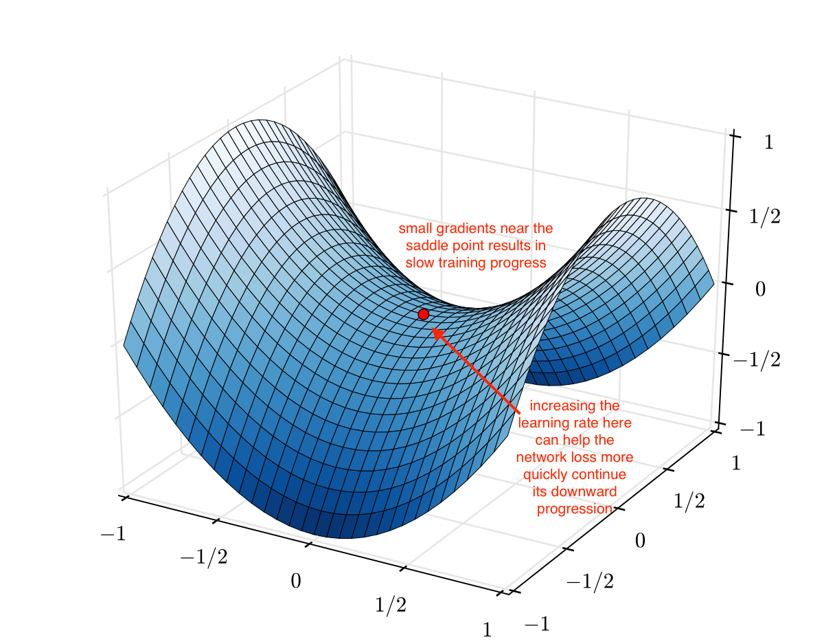
- Increasing the learning rate can also allow for “more rapid traversal of saddle point plateaus. As you can see in the image below, the gradients can be very small at a saddle point. Because the parameter updates are a function of the gradient, this results in our optimization taking very small steps; it can be useful to increase the learning rate here to avoid getting stuck for too long at a saddle point. So periodic increase in learning rate can help in quickly jumping saddle points.
The codes for cyclic learning rate can be found here.
As an end note, there is no single leanring rate schedule scheme that works best for all applications and architectures. I almost always start my experiments with the linear decay scheme (decaying the learning rate until some iteration and then keeping it constant). You can always start with some scheme and if the training error doesn’t go down as expected, try some other scheme. Happy coding.